
Halley’s Comet (Figure \(\PageIndex\)) orbits the sun about once every \(75\) years. Its path can be considered to be a very elongated ellipse. Other comets follow similar paths in space. These orbital paths can be studied using systems of equations. These systems, however, are different from the ones we considered in the previous section because the equations are not linear.

Figure \(\PageIndex\): Halley’s Comet (credit: "NASA Blueshift"/Flickr)
In this section, we will consider the intersection of a parabola and a line, a circle and a line, and a circle and an ellipse. The methods for solving systems of nonlinear equations are similar to those for linear equations.
A system of nonlinear equations is a system of two or more equations in two or more variables containing at least one equation that is not linear. Recall that a linear equation can take the form \(Ax+By+C=0\). Any equation that cannot be written in this form in nonlinear. The substitution method we used for linear systems is the same method we will use for nonlinear systems. We solve one equation for one variable and then substitute the result into the second equation to solve for another variable, and so on. There is, however, a variation in the possible outcomes.
There are three possible types of solutions for a system of nonlinear equations involving a parabola and a line.
Figure \(\PageIndex\) illustrates possible solution sets for a system of equations involving a parabola and a line.
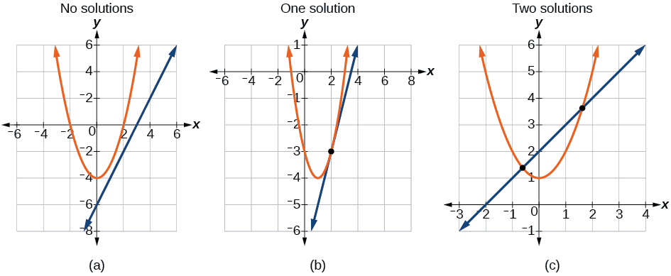
Figure \(\PageIndex\)
Solve the system of equations.
\[\begin x−y &= −1\nonumber \\ y &= x^2+1 \nonumber \end\]
Solution
Solve the first equation for \(x\) and then substitute the resulting expression into the second equation.
Expand the equation and set it equal to zero.
\[ \begin y & =^2+1\nonumber \\ &=(y^2−2y+1)+1\nonumber \\ &=y^2−2y+2\nonumber \\ 0 &= y^2−3y+2\nonumber \\ &= (y−2)(y−1) \nonumber \end\]
Solving for \(y\) gives \(y=2\) and \(y=1\). Next, substitute each value for \(y\) into the first equation to solve for \(x\). Always substitute the value into the linear equation to check for extraneous solutions.
\[\begin x−y &=−1\nonumber \\ x−(2) &= −1\nonumber \\ x &= 1\nonumber \\ x−(1) &=−1\nonumber \\ x &= 0 \nonumber \end\]
The solutions are \((1,2)\) and \((0,1)\),which can be verified by substituting these \((x,y)\) values into both of the original equations (Figure \(\PageIndex\)).
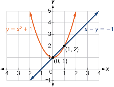
Figure \(\PageIndex\)
Yes, but because \(x\) is squared in the second equation this could give us extraneous solutions for \(x\).
\[\begin y &= x^2+1\nonumber \\ y &= x^2+1\nonumber \\ x^2 &= 0\nonumber \\ x &= \pm \sqrt=0 \nonumber \end\]
This gives us the same value as in the solution.
\[\begin y &= x^2+1\nonumber \\ 2 &= x^2+1\nonumber \\ x^2 &= 1\nonumber \\ x &= \pm \sqrt=\pm 1 \nonumber \end\]
Notice that \(−1\) is an extraneous solution.
Solve the given system of equations by substitution.
\[\begin 3x−y &= −2\nonumber \\ 2x^2−y &= 0 \nonumber \end\]
Just as with a parabola and a line, there are three possible outcomes when solving a system of equations representing a circle and a line.
Figure \(\PageIndex\) illustrates possible solution sets for a system of equations involving a circle and a line.
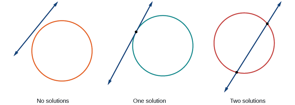
Figure \(\PageIndex\)
Find the intersection of the given circle and the given line by substitution.
\[\begin x^2+y^2 &= 5\nonumber \\ y &= 3x−5 \nonumber \end\]
Solution
One of the equations has already been solved for \(y\). We will substitute \(y=3x−5\) into the equation for the circle.
\[\begin x^2+^2 &= 5\nonumber \\ x^2+9x^2−30x+25 &= 5\nonumber \\ 10x^2−30x+20 &= 0 \end \]
Now, we factor and solve for \(x\).
\[\begin 10(x2−3x+2) &= 0\nonumber \\ 10(x−2)(x−1) &= 0\nonumber \\ x &= 2\nonumber \\ x &= 1 \nonumber \end\]
Substitute the two \(x\)-values into the original linear equation to solve for \(y\).
\[\begin y &= 3(2)−5\nonumber \\ &= 1\nonumber \\ y &= 3(1)−5\nonumber \\ &= −2 \nonumber \end\]
The line intersects the circle at \((2,1)\) and \((1,−2)\),which can be verified by substituting these \((x,y)\) values into both of the original equations (Figure \(\PageIndex\)).
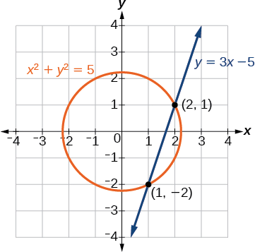
Figure \(\PageIndex\)
Solve the system of nonlinear equations.
\[\begin x^2+y^2 &= 10\nonumber \\ x−3y &= −10 \nonumber \end\]
We have seen that substitution is often the preferred method when a system of equations includes a linear equation and a nonlinear equation. However, when both equations in the system have like variables of the second degree, solving them using elimination by addition is often easier than substitution. Generally, elimination is a far simpler method when the system involves only two equations in two variables (a two-by-two system), rather than a three-by-three system, as there are fewer steps. As an example, we will investigate the possible types of solutions when solving a system of equations representing a circle and an ellipse.
Figure \(\PageIndex\) illustrates possible solution sets for a system of equations involving a circle and an ellipse.
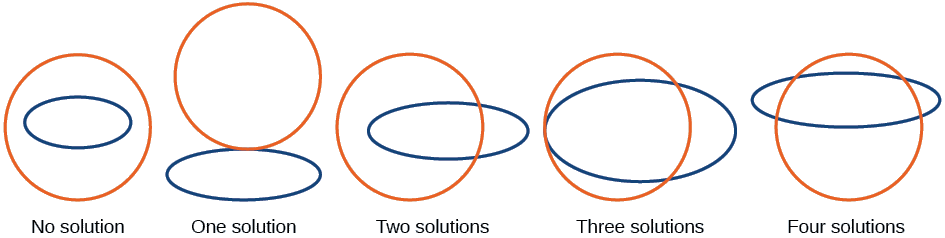
Figure \(\PageIndex\)
Solve the system of nonlinear equations.
\[\begin x^2+y^2 &= 26 &(1)\nonumber \\ 3x^2+25y^2 &= 100 & (2) \nonumber \end\]
Solution
Let’s begin by multiplying equation (1) by \(−3\),and adding it to equation (2).
\[\begin (−3)(x^2+y^2) = (−3)(26)&\nonumber \\ −3x^2−3y^2 = −78 &\nonumber \\ \underline&\nonumber \\ 22y^2=22& \nonumber \end\]
After we add the two equations together, we solve for \(y\).
\[\begin y^2 &= 1\nonumber \\ y &= \pm \sqrt=\pm 1 \nonumber \end\]
Substitute \(y=\pm 1\) into one of the equations and solve for \(x\).
\[\begin x^2+^2 &= 26\nonumber \\ x^2+1 &= 26\nonumber \\ x^2 &= 25\nonumber \\ x &= \pm \sqrt=\pm 5\nonumber \\ x^2+^2 &= 26\nonumber \\ x^2+1 &= 26\nonumber \\ x^2 &= \pm \sqrt=\pm 5 \nonumber \end\]
There are four solutions: \((5,1)\), \((−5,1)\), \((5,−1)\),and \((−5,−1)\). See Figure \(\PageIndex\).
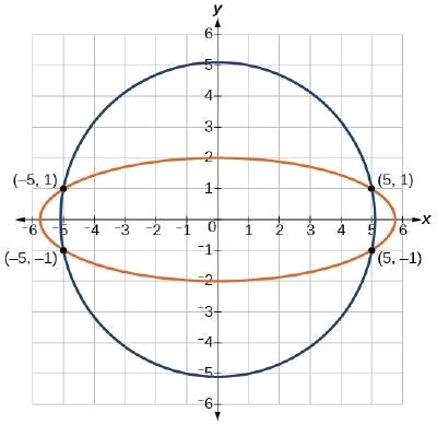
Figure \(\PageIndex\)
Find the solution set for the given system of nonlinear equations.
\[\begin 4x^2+y^2 &= 13\nonumber \\ x^2+y^2 &= 10 \nonumber \end\]
All of the equations in the systems that we have encountered so far have involved equalities, but we may also encounter systems that involve inequalities. We have already learned to graph linear inequalities by graphing the corresponding equation, and then shading the region represented by the inequality symbol. Now, we will follow similar steps to graph a nonlinear inequality so that we can learn to solve systems of nonlinear inequalities. A nonlinear inequality is an inequality containing a nonlinear expression. Graphing a nonlinear inequality is much like graphing a linear inequality.
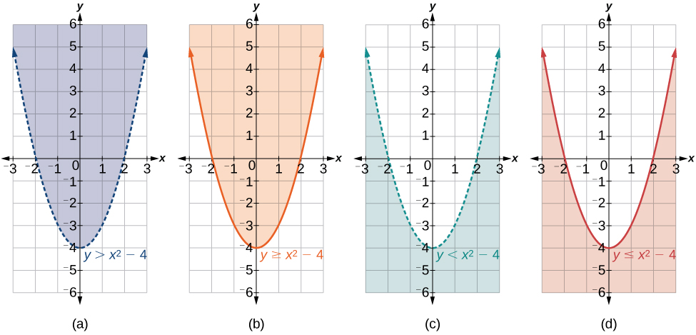
Figure \(\PageIndex\): (a) an example of \(y>a\); (b) an example of \(y≥a\); (c) an example of \(y
Graph the inequality \(y>x^2+1\).
Solution
First, graph the corresponding equation \(y=x^2+1\). Since \(y>x^2+1\) has a greater than symbol, we draw the graph with a dashed line. Then we choose points to test both inside and outside the parabola. Let’s test the points
\((0,2)\) and \((2,0)\). One point is clearly inside the parabola and the other point is clearly outside.
\[\begin y &> x^2+1\nonumber \\ 2 &> (0)^2+1\nonumber \\ 2 &>1 & \text\nonumber \\\nonumber \\\nonumber \\ 0 &> (2)^2+1\nonumber \\ 0 &> 5 & \text \nonumber \end\]
The graph is shown in Figure \(\PageIndex\). We can see that the solution set consists of all points inside the parabola, but not on the graph itself.
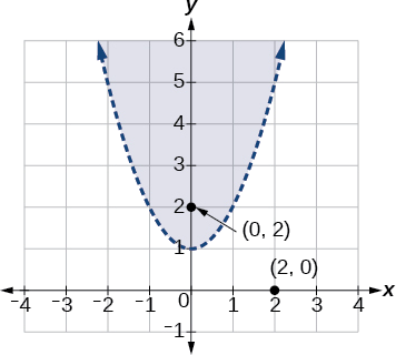
Figure \(\PageIndex\)
Now that we have learned to graph nonlinear inequalities, we can learn how to graph systems of nonlinear inequalities. A system of nonlinear inequalities is a system of two or more inequalities in two or more variables containing at least one inequality that is not linear. Graphing a system of nonlinear inequalities is similar to graphing a system of linear inequalities. The difference is that our graph may result in more shaded regions that represent a solution than we find in a system of linear inequalities. The solution to a nonlinear system of inequalities is the region of the graph where the shaded regions of the graph of each inequality overlap, or where the regions intersect, called the feasible region.
Graph the given system of inequalities.
\[\begin x^2−y &≤ 0\nonumber \\ 2x^2+y &≤ 12 \nonumber \end\]
Solution
These two equations are clearly parabolas. We can find the points of intersection by the elimination process: Add both equations and the variable \(y\) will be eliminated. Then we solve for \(x\).
\[\begin x^2−y = 0&\nonumber \\ \underline&\nonumber \\ 3x^2=12&\nonumber \\ x^2=4 &\nonumber \\ x=\pm 2 & \nonumber \end\]
Substitute the \(x\)-values into one of the equations and solve for \(y\).
\[\begin x^2−y &= 0\nonumber \\ ^2−y &= 0\nonumber \\ 4−y &= 0\nonumber \\ y &= 4\nonumber \\\nonumber \\ ^2−y &= 0\nonumber \\ 4−y &= 0\nonumber \\ y &= 4 \nonumber \end\]
The two points of intersection are \((2,4)\) and \((−2,4)\). Notice that the equations can be rewritten as follows.
\[\begin x^2-y & ≤ 0\nonumber \\ x^2 &≤ y\nonumber \\ y &≥ x^2\nonumber \\\nonumber \\\nonumber \\ 2x^2+y &≤ 12\nonumber \\ y &≤ −2x^2+12 \nonumber \end\]
Graph each inequality. See Figure \(\PageIndex\). The feasible region is the region between the two equations bounded by \(2x^2+y≤12\) on the top and \(x^2−y≤0\) on the bottom.
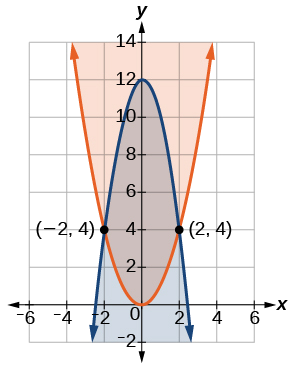
Figure \(\PageIndex\)
Graph the given system of inequalities.
\[\begin y &≥ x^2−1\nonumber \\ x−y &≥ −1 \nonumber \end\]
Shade the area bounded by the two curves, above the quadratic and below the line.
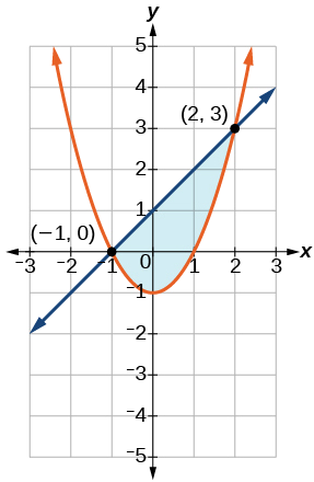
Figure \(\PageIndex\)
Access these online resources for additional instruction and practice with nonlinear equations.
This page titled 7.4: Systems of Nonlinear Equations and Inequalities - Two Variables is shared under a CC BY 4.0 license and was authored, remixed, and/or curated by OpenStax via source content that was edited to the style and standards of the LibreTexts platform.